A Sample Space Perspective on Flow Matching
Published:
A Sample Space Perspective on Flow Matching
Introduction
Flow matching, introduced by Lipman et al. in Flow Matching for Generative Modeling, has become one of the central ideas behind modern flow-based generative models. Closely related rectified-flow methods now appear in large-scale systems such as Stable Diffusion 3 and FLUX.1.
Despite being formally correct, I often found the standard presentation hard to follow. One usually starts with a path of probability distributions, introduces a velocity field through a continuity equation, and only later arrives at a tractable training objective. Along the way, auxiliary variables may appear as an additional device that makes the objective tractable.
From the sample-space point of view, these auxiliary variables are not a separate trick. They are simply part of how we choose to construct the random path. What matters is not whether the path was built from endpoints alone or from endpoints together with extra randomness. What matters is that we can sample $X_t$ and compute its pathwise derivative $\dot X_t$. Once we can do that, the velocity field is the conditional average of this derivative.
In this post, I want to show how the usual flow matching machinery can be derived naturally from a sample-path perspective, where the construction is more direct.
The guiding idea is simple. A deterministic curve connecting two points can be turned into a random path by randomizing its endpoints. Taking laws along this random path then gives an explicit path of probability measures, connecting a simple source distribution $\mu_0$ chosen by us to a target distribution $\mu_1$ observed through samples.
From Curves to Random Paths
Let us start with the deterministic case. Suppose we are given two points
\[x_0, x_1 \in \mathbb{R}^d.\]A path connecting them is a map
\[\gamma : [0,1] \times \mathbb{R}^d \times \mathbb{R}^d \to \mathbb{R}^d,\]such that
\[\gamma(0, x_0, x_1) = x_0, \qquad \gamma(1, x_0, x_1) = x_1.\]For example, the linear path is given by
\[\gamma(t, x_0, x_1) = (1-t)x_0 + t x_1.\]Now comes the simple but important step: we replace the deterministic endpoints by random variables.
Let
\[X_0 \sim \mu_0, \qquad X_1 \sim \mu_1,\]where $\mu_0$ is the source distribution and $\mu_1$ is the target distribution. We then define
\[X_t := \gamma(t, X_0, X_1).\]This is a random path. At each time $t$, it has a law:
\[\mu_t := \operatorname{Law}(X_t).\]In this way, the deterministic curve $\gamma$ induces a path of probability measures
\[(\mu_t)_{t \in [0,1]}\]connecting $\mu_0$ and $\mu_1$.
There is one subtle point hidden here. To construct the random pair $(X_0, X_1)$, we must choose a coupling of $\mu_0$ and $\mu_1$, that is, a joint distribution $\pi$ on $\mathbb{R}^d \times \mathbb{R}^d$ with marginals $\mu_0$ and $\mu_1$. Then
\[(X_0, X_1) \sim \pi.\]Different choices of $\pi$ lead to different random paths, and therefore to different probability paths $(\mu_t)$. The most basic choice is the independent coupling
\[\pi = \mu_0 \otimes \mu_1,\]which simply samples $X_0$ and $X_1$ independently.
This is already enough to define a bridge from $\mu_0$ to $\mu_1$ explicitly.
The Continuity Equation
We now take a short excursion into the mathematical object that connects particle dynamics with the evolution of probability measures.
Suppose we are given a time-dependent velocity field
\[v_t : \mathbb{R}^d \to \mathbb{R}^d.\]If we initialize a particle randomly,
\[Y_0 \sim \mu_0,\]and move it according to the ordinary differential equation
\[\frac{d}{dt}Y_t = v_t(Y_t),\]then the particle remains random at all later times. We denote its law by
\[\nu_t := \operatorname{Law}(Y_t).\]The continuity equation describes the evolution of this probability path. If $\nu_t$ has density $p_t$, then the equation is
\[\partial_t p_t(x) + \nabla \cdot \big(p_t(x) v_t(x)\big) = 0.\]This equation expresses conservation of mass. Probability does not disappear or get created; it only moves through space.
Equivalently, in measure notation, one writes
\[\partial_t \nu_t + \nabla \cdot(\nu_t v_t) = 0.\]A convenient way to read the same equation is in weak form. For every smooth test function $\varphi : \mathbb{R}^d \to \mathbb{R}$,
\[\frac{d}{dt} \int_{\mathbb{R}^d} \varphi(x) \, d\nu_t(x) = \int_{\mathbb{R}^d} \nabla \varphi(x) \cdot v_t(x) \, d\nu_t(x).\]This weak formulation is often the cleanest way to reason about flow matching, because it does not require us to manipulate densities directly.
The relationship between paths, velocity fields, and the continuity equation has two sides.
First, if the ODE is well posed, then the laws of its solutions solve the continuity equation. In other words, the randomly initialized ODE produces a path of probability measures, and this path satisfies the PDE above.
Second, under suitable regularity assumptions, the converse viewpoint is also available. Given a sufficiently regular path of probability measures $(\mu_t)_{t \in [0,1]}$, one can find a velocity field $v_t$ such that
\[\partial_t \mu_t + \nabla \cdot(\mu_t v_t) = 0.\]This velocity field is generally not unique. There may be several different velocity fields that realize the same path of probability measures.
The important point is not uniqueness of the velocity field. The important point is uniqueness of the evolution once a velocity field has been chosen. If, for a particular compatible velocity field $v_t$, the continuity equation with initial condition $\mu_0$ is well posed, then the path $(\mu_t)$ is the unique solution of
\[\partial_t \nu_t + \nabla \cdot(\nu_t v_t) = 0, \qquad \nu_0 = \mu_0.\]This is the result we will use. We will construct a reference path $(\mu_t)$ explicitly, then write down a velocity field $v_t$ that makes this path solve the continuity equation. The randomly initialized ODE with the same velocity field also gives a solution to the same continuity equation. By uniqueness, both probability paths must agree.
The endpoint is therefore not imposed a second time during sampling. It is already encoded in the reference path. Once the velocity field and initial condition uniquely determine that same path, the terminal distribution follows automatically.
The Continuity Equation for Flow Matching
We now return to our explicit random path. We have constructed
\[\mu_t := \operatorname{Law}(X_t), \qquad X_0 \sim \mu_0, \qquad X_1 \sim \mu_1.\]Thus the endpoints are fixed by construction:
\[\mu_0 = \operatorname{Law}(X_0), \qquad \mu_1 = \operatorname{Law}(X_1).\]Assume that $X_t$ is differentiable in time. Its pathwise velocity is
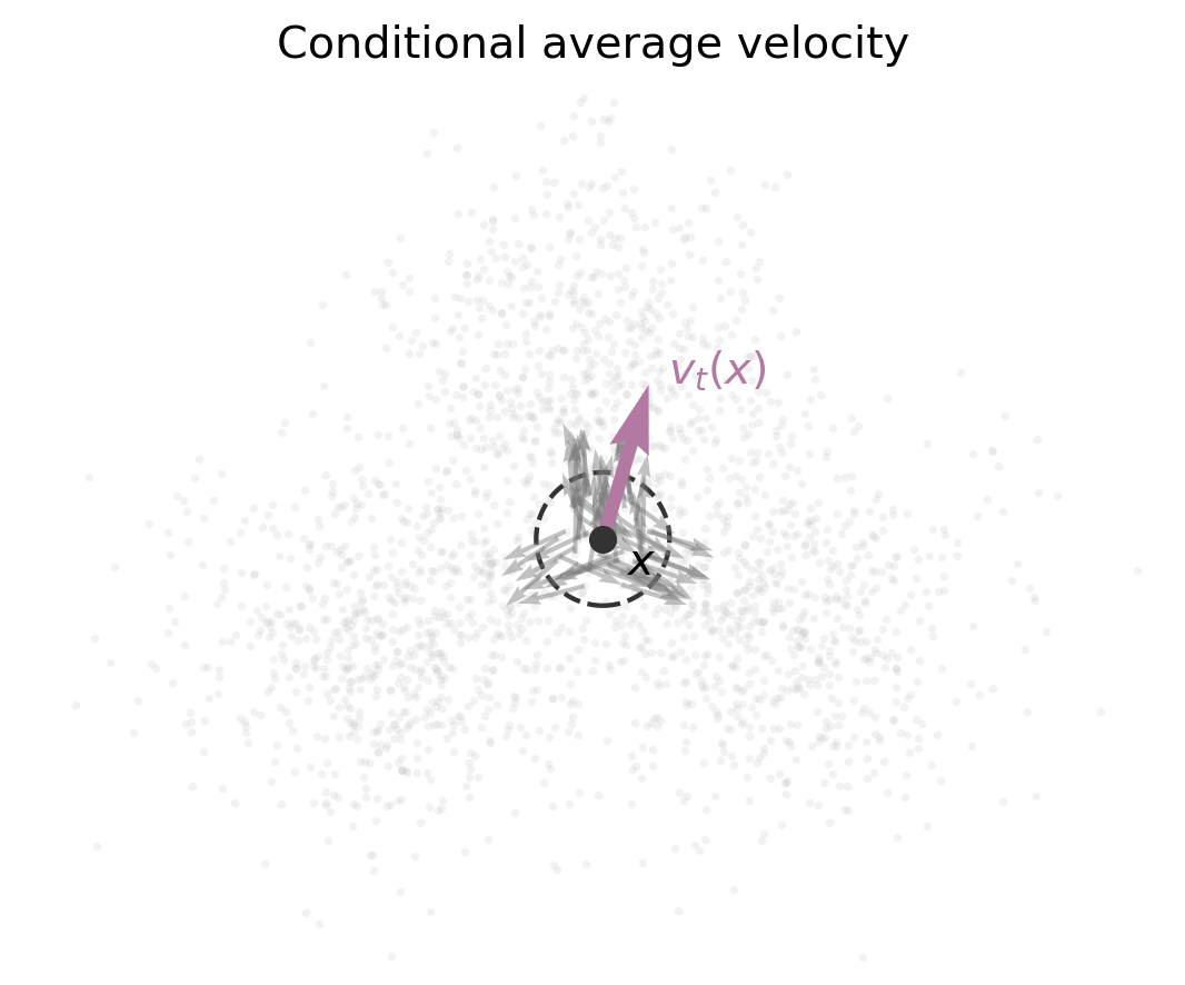
\[\dot{X}_t := \frac{d}{dt}X_t.\]This is a random vector. If we observe that a particle is located at $x$ at time $t$, we do not necessarily know which path it came from. Many paths may pass through the same point, with different instantaneous velocities.
The flow-matching velocity field is the average velocity of all paths passing through $x$ at time $t$:
We now verify that this field realizes the path $\mu_t$ through the continuity equation.
Take a smooth test function $\varphi$. Since $\mu_t = \operatorname{Law}(X_t)$,
\[\int_{\mathbb{R}^d} \varphi(x) \, d\mu_t(x) = \mathbb{E}[\varphi(X_t)].\]Differentiating in time gives
\[\frac{d}{dt}\mathbb{E}[\varphi(X_t)] = \mathbb{E}[\nabla \varphi(X_t) \cdot \dot{X}_t].\]Now use the defining property of conditional expectation:
\[\mathbb{E}[\nabla \varphi(X_t) \cdot \dot{X}_t] = \mathbb{E} \left[ \nabla \varphi(X_t) \cdot \mathbb{E}[\dot{X}_t \mid X_t] \right].\]By definition of $v_t$, this is
\[\mathbb{E}[\nabla \varphi(X_t) \cdot v_t(X_t)] = \int_{\mathbb{R}^d} \nabla \varphi(x) \cdot v_t(x) \, d\mu_t(x).\]Hence
\[\frac{d}{dt} \int_{\mathbb{R}^d} \varphi(x) \, d\mu_t(x) = \int_{\mathbb{R}^d} \nabla \varphi(x) \cdot v_t(x) \, d\mu_t(x),\]which is precisely the weak form of the continuity equation.
So the conditional-average velocity field
\[v_t(x) = \mathbb{E}[\dot{X}_t \mid X_t = x]\]satisfies
\[\partial_t \mu_t + \nabla \cdot(\mu_t v_t) = 0\]for the probability path induced by the random path $X_t$.
This is the precise bridge from the explicit path construction to a sampling procedure. Under the usual well-posedness assumptions, if we solve
\[\frac{d}{dt}Y_t = v_t(Y_t), \qquad Y_0 \sim \mu_0,\]then the law of $Y_t$ solves the same continuity equation with the same initial condition as $\mu_t$. By uniqueness,
\[\operatorname{Law}(Y_t) = \mu_t\]for all $t \in [0,1]$. In particular,
\[Y_1 \sim \mu_1.\]This is why learning the velocity field is enough: once the field is known, sampling is just ODE integration from the source distribution.
Learning the Velocity Field
We have now reduced the problem to learning a velocity field. If we knew $v_t$ for every $t \in [0,1]$, then sampling would be straightforward: draw $Y_0 \sim \mu_0$ and solve the ODE
\[\frac{d}{dt}Y_t = v_t(Y_t).\]In practice, of course, we do not know $v_t$. We approximate the entire time-dependent vector field by a neural network
\[u_\theta(t,x) \approx v_t(x).\]A natural objective would be to choose $\theta$ so that $u_\theta$ is close to $v_t$ along the whole probability path. For example, one could consider the integrated $L^2$ loss
\[\mathcal{L}_{\mathrm{ideal}}(\theta) := \int_0^1 \mathbb{E} \left[ \left\| u_\theta(t, X_t) - v_t(X_t) \right\|^2 \right] \, dt.\]Here the expectation is over the randomness of $X_t$ at a fixed time $t$. More generally, any loss whose unique minimizer is the full field $(v_t)_{t \in [0,1]}$ would serve the same conceptual purpose. The integrated $L^2$ loss is just the most direct choice.
Mathematically, this objective is obvious. It says: learn the velocity field by matching the velocity field. But it is not tractable, because it contains the unknown target $v_t$.
The crucial observation is that we can replace this intractable target by the pathwise velocity $\dot{X}_t$. Define
\[\mathcal{L}_{\mathrm{FM}}(\theta) := \int_0^1 \mathbb{E} \left[ \left\| u_\theta(t, X_t) - \dot{X}_t \right\|^2 \right] \, dt,\]where the expectation is again over the random path at fixed time $t$.
Why does this work? Because conditional expectation is an $L^2$ projection.
Projection theorem. Let $Y$ be a square-integrable random vector and let $Z$ be another random variable. Among all functions $f(Z)$, the unique minimizer of
\[\mathbb{E}\left[\|f(Z)-Y\|^2\right]\]is
\[f^*(Z) = \mathbb{E}[Y \mid Z].\]Apply this with
\[Y = \dot{X}_t, \qquad Z = X_t.\]For each fixed time $t$, the minimizer of
\[\mathbb{E} \left[ \left\| u(t, X_t) - \dot{X}_t \right\|^2 \right]\]is
\[u^*(t,x) = \mathbb{E}[\dot{X}_t \mid X_t = x] = v_t(x).\]Thus, for every fixed time $t$, regressing onto the pathwise velocity recovers the desired velocity field $v_t$. Integrating over time then recovers the whole time-dependent field $(v_t)_{t \in [0,1]}$.
This is the key step that makes flow matching tractable. The ideal target $v_t(X_t)$ is unknown, but the regression target $\dot{X}_t$ is easy to compute because we chose the path explicitly.
The Linear Path
The simplest construction is the linear path. Sample
\[(X_0, X_1) \sim \pi,\]where $\pi$ is a coupling of $\mu_0$ and $\mu_1$, and define
\[X_t = (1-t)X_0 + tX_1.\]Then
\[\dot{X}_t = X_1 - X_0.\]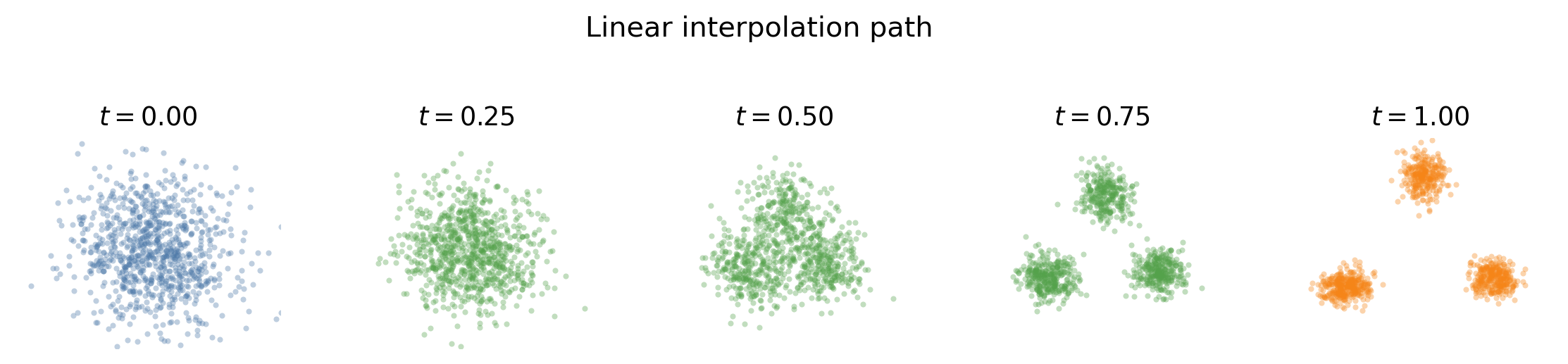
The corresponding velocity field is
\[v_t(x) = \mathbb{E}[X_1 - X_0 \mid X_t = x].\]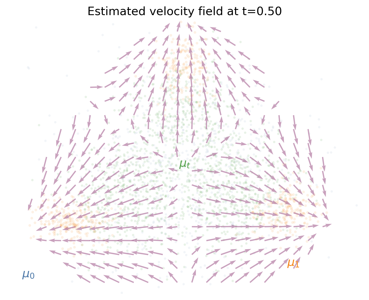
The training objective becomes
\[\mathcal{L}_{\mathrm{FM}}(\theta) = \mathbb{E} \left[ \left\| u_\theta(t, (1-t)X_0 + tX_1) - (X_1 - X_0) \right\|^2 \right].\]This is already a complete flow matching method. We sample a source point, sample a data point, choose a time, interpolate between them, and regress onto the velocity of the interpolation.
The Role of Auxiliary Variables
Auxiliary variables sometimes make flow matching presentations feel more complicated than necessary. From the present point of view, they are not mysterious. They are simply additional random quantities that help us define more flexible paths in sample space.
For example, suppose we introduce an auxiliary random variable $Z$ and define
\[X_t = \gamma(t, X_0, X_1, Z).\]As long as the endpoints satisfy
\[X_0 \sim \mu_0, \qquad X_1 \sim \mu_1,\]this still defines a path of probability measures through
\[\mu_t = \operatorname{Law}(X_t).\]The only thing we need for the flow matching construction is that we can differentiate the path pointwise in time. If $\dot{X}_t$ is available, then the same formula gives the associated velocity field:
\[v_t(x) = \mathbb{E}[\dot{X}_t \mid X_t = x].\]Thus auxiliary variables are not a separate principle. They are part of the path construction. Once the random path is defined, the induced probability path and the velocity field are obtained in exactly the same way as before.
The Gaussian conditional path is an important example. Let
\[Z \sim \mathcal{N}(0,I_d), \qquad Y \sim \mu_1,\]with $Z$ and $Y$ independent. Here $Y$ denotes a data sample. Choose scalar schedules $a_t$ and $\sigma_t$ and define
\[X_t = \gamma(t,Z,Y) := a_t Y + \sigma_t Z.\]Conditional on the data point $Y$, this gives
\[X_t \mid Y \sim \mathcal{N}(a_t Y, \sigma_t^2 I_d).\]To connect a standard Gaussian source to the data distribution, we choose the endpoint conditions
\[a_0 = 0, \qquad \sigma_0 = 1, \qquad a_1 = 1, \qquad \sigma_1 = 0.\]Then
\[X_0 = Z \sim \mathcal{N}(0,I_d), \qquad X_1 = Y \sim \mu_1.\]The pathwise velocity is again explicit:
\[\dot{X}_t = \dot{a}_t Y + \dot{\sigma}_t Z.\]So the same recipe still applies:
- sample the variables needed to construct $X_t$,
- compute the pathwise velocity $\dot{X}_t$,
- train $u_\theta(t,X_t)$ to predict $\dot{X}_t$.
For the simple choice $a_t=t$ and $\sigma_t=1-t$, this reduces to the linear interpolation between Gaussian noise and data:
\[X_t = tY + (1-t)Z.\]More general schedules give different Gaussian conditional paths, but the principle does not change. Auxiliary variables are just a way to write down richer random paths explicitly.
Sampling from the Learned Flow
After training, we generate new samples by solving an ordinary differential equation. We start from a fresh sample
\[Y_0 \sim \mu_0\]and evolve it according to
\[\frac{d}{dt}Y_t = u_\theta(t, Y_t), \qquad t \in [0,1].\]If $u_\theta$ is close to the true velocity field $v_t$, then the law of $Y_t$ approximately follows the path $\mu_t$. In particular, the terminal point $Y_1$ should be approximately distributed according to $\mu_1$.
This is the final generative procedure:
Sample from the simple source distribution, then flow the sample through the learned velocity field until it reaches the target distribution.
Conclusion
The first-principles view of flow matching is very compact.
We start with a deterministic way to connect two points. By randomizing the endpoints, this becomes a random path connecting a source distribution $\mu_0$ to a target distribution $\mu_1$. Taking laws at intermediate times gives a path of probability measures. The associated velocity field is the average pathwise velocity of all particles passing through a point:
\[v_t(x) = \mathbb{E}[\dot{X}_t \mid X_t = x].\]The continuity equation tells us that this velocity field transports the intermediate distributions. The $L^2$ projection theorem tells us that we can learn the field by regressing directly onto the pathwise velocity:
\[u_\theta(t,X_t) \approx \dot{X}_t.\]This is the central mechanism of flow matching. Different versions of the method come from different choices of the random path, but the underlying idea remains the same: construct the bridge explicitly, then learn its velocity.